How did Lula turn around the 2026 Presidential Election?
TL;DR
Without individual-level information we can’t be sure, but analysis of the available data suggests that Lula won because people who voted for third candidates or spoiled their ballot in the first round voted tactically to keep Bolsonaro out.

Lula’s shock re-election on 25 October followed a first-round loss, in which Flávio Bolsonaro won 47% of the vote to Lula’s 45%. Bolsonaro led the opinion polls right up to election day and between-round polling suggested he’d get most of the third-candidate votes. But to many people’s surprise, we woke up to news that Lula had gained 10M votes in the second round, and won with 51.8% of the vote.
It was the first time in Brazilian democratic history that a presidential candidate had won the second round after losing the first. Early write-ups of the election pointed to an energetic between-round campaign by Lula’s supporters, with rallies attended by millions, key “clippable” moments in the TV debates, and late spending promises by the incumbent president.
In particular, there has been a lot of focus on the grassroots online campaigns run by Lula’s supporters. Most notably, André Janones, an allied1 member of the Câmara dos Deputados, ran a WhatsApp channel called “Exército do Lula” (Lula’s Army) (Dyer, Pooler, and Beatriz 2026). It broadcast mobilisation messages to over 11M supporters, encouraging them to share social media posts to boost pro-Lula content in the algorithms. Alexandre Afonso has written an excellent blog post analysing the content of the channel.
In his book Prototype Politics, Kreiss (2016) describes election post-mortems as a social process of “meaning-making”, in which particular elements of a campaign are picked out and narratives emerge that these elements “won” (or lost) the election. In short, we all tend to pick out particular elements of a campaign and attribute its success to them.
In reality, working out why a campaign won is very challenging. Among political scientists, there is a long-running and unresolved debate about whether campaign periods matter at all for election outcomes, and even if they do, isolating the effects of particular interventions requires careful research design (Foos and Metson 2026).
Nonetheless, the sheer scale of the mobilisation achieved warrants some exploration. Beyond the “Exército do Lula” WhatsApp mobilisation, other smaller initiatives shed some light on the nature of the between-round campaign. In particular, the webpage “Onde dá pra conversar” (Where you can have a conversation) showed which areas could be swung towards Lula and encouraged voters to reach out to their neighbours to persuade and mobilise them. This tactic echoes the decentralised “relational organising” popularised by Obama’s 2012 campaign (McKenna and Han 2014).
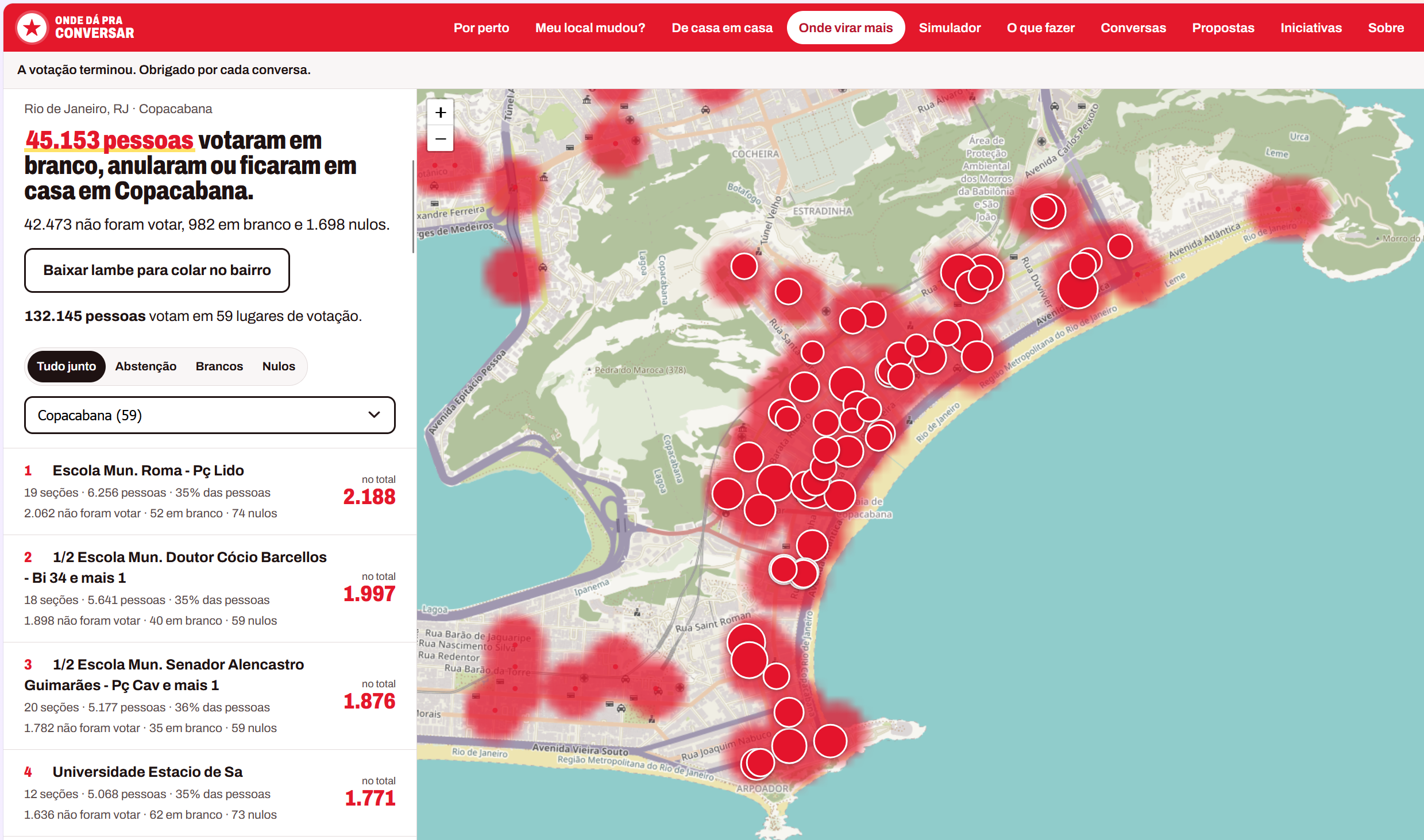
The site highlighted polling sections (seções de votação) where the number of abstentions and invalid votes was larger than the gap between Lula and Bolsonaro. It also offered detailed suggested scripts for talking to voters who had abstained, spoiled their ballot or voted for another candidate in the first round.
Political scientists may be interested to learn that the advice on persuasion appears to draw very closely on the logic of “deep canvassing” interventions tested in a series of experiments in the US (Broockman and Kalla 2016; Kalla and Broockman 2023):
How to start the conversation
- Begin by acknowledging what the other person likes about their chosen candidate. People lower their guard when they feel respected.
- Highlight common ground by placing two excerpts side by side. Each includes its source and page number: just tap to view.
- Avoid speaking ill of their candidate. Like you, they want a better country. The question now is: who is best placed to take that forward on the 25th?
- If they don’t reach a decision right away, that’s perfectly fine. Thank them and leave the door open. Deciding how to vote takes time.
Beyond persuasion, supporters of Lula’s party, the Workers’ Party (Partido dos Trabalhadores, PT) placed a strong emphasis on mobilising people who hadn’t voted in the first round. At first this might seem puzzling: Brazil has compulsory voting for much of the population (literate adults aged 18–70). Even so, turnout does vary. For voters over 70 and illiterate voters, voting is voluntary. Voters can also justify their absence, and the penalty for not voting is small: usually around R$3.51 (US$0.70), though it can be up to R$35 for wealthier voters (Morales 2026).
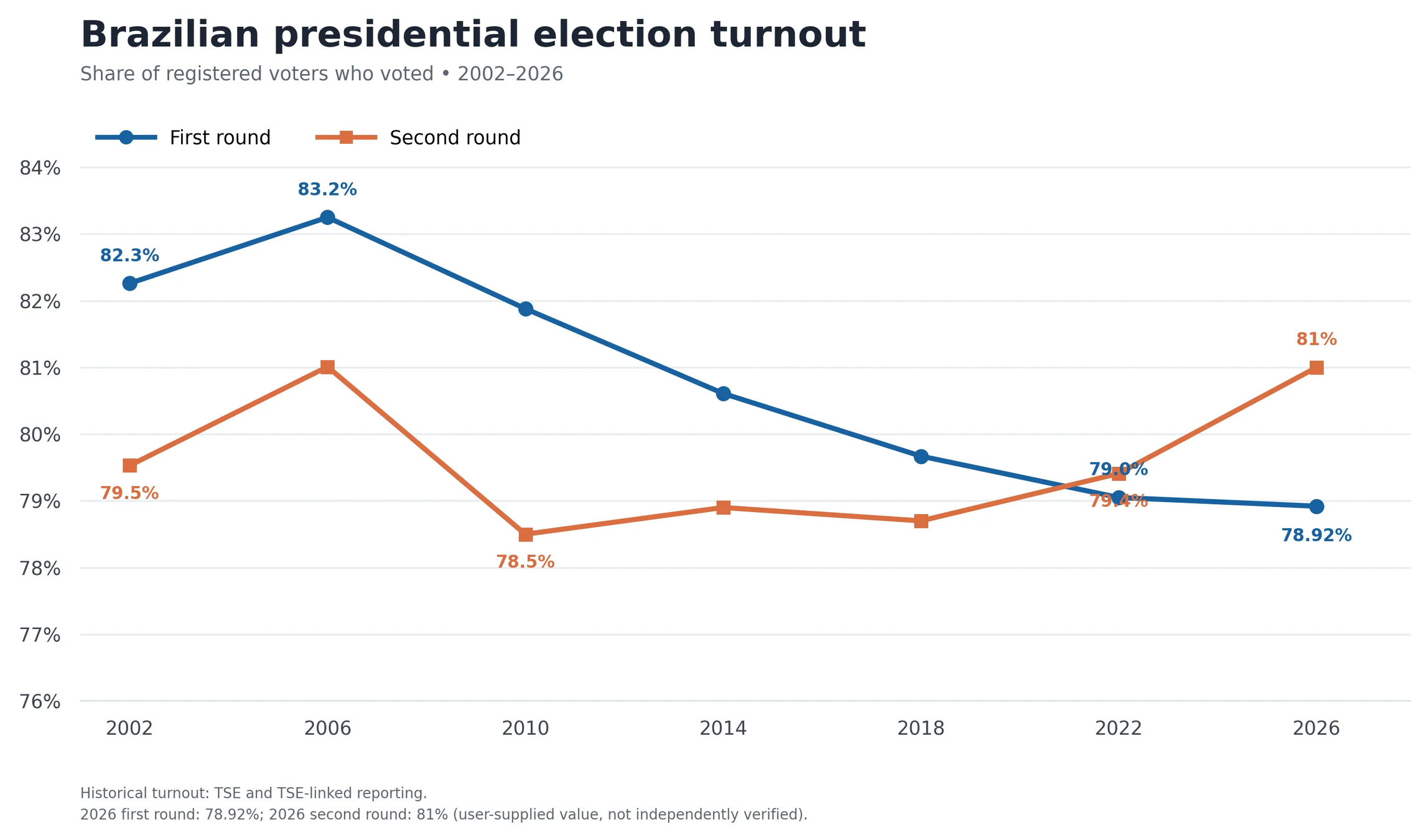
On the surface, mobilisation appears to have played a major role in this election: the first round saw the lowest first-round turnout since 2002, and turnout increased substantially in the second round (Figure 1).
Analyses of where Lula gained the most votes between rounds suggest that Lula won by gaining voters in areas that we wouldn’t typically expect to vote for the PT (see posts by Juan Machado and Owen Winter). This doesn’t fit comfortably with a pure mobilisation story, where we’d expect generally supportive areas to have been where gains were strongest.
To dig into this more, I use section-level data to describe how the election played out between the two rounds, and to see what we can learn about how Lula achieved his historic win. Seções de votação (polling sections) are the smallest unit at which results are reported. Each is a single urna eletrônica (voting machine), to which around 300 voters are assigned (μ=318, σ=66).
What did Lula need to win?
Before exploring how Lula won, it’s worth outlining the scale of the challenge as it looked before the second round.
Figure 2 shows the results of the first round, using all registered voters as the denominator. Lula trailed Bolsonaro by 2.2M votes. 21.1% of registered voters abstained, 5.9% voted for third candidates and 3.8% spoiled their ballot.2
No candidate reached 50% of valid votes, triggering a runoff between Bolsonaro and Lula. After the first round, most of the other candidates endorsed one of the two runoff candidates. Five endorsed Bolsonaro, three Lula and two remained neutral or endorsed a null vote (sources in Table 1).
The left panel of Figure 3 shows the third-candidate vote grouped by whom each candidate endorsed in the second round. If every third-candidate voter had followed their candidate’s endorsement, Bolsonaro could have counted on 6.4M additional votes, and Lula on just under 200K.
However, a poll of 2,154 voters conducted by Quaest suggested that third-candidate voters wouldn’t necessarily follow their candidate’s endorsement.
The right panel of Figure 3 shows how many votes each runoff candidate would have received according to this poll (see the appendix for more details). Even with some voters not following their candidate’s endorsement, Lula would still win 1.1M fewer of these votes than Bolsonaro.
Adding these (very rough) projected vote transfers to the first-round votes3, Figure 4 demonstrates how weak Lula’s position looked before the second round. Based on the information available at the time, a back-of-the-envelope projection would have had Lula trailing Bolsonaro by 3M votes.
To be explicit, the path to turning it around in the second round was steep, but certainly not “impossible” as a certain recently-US-based Brazilian presidential candidate claimed. Excluding both candidates’ first-round voters, there was a pool of nearly 50M voters from which Lula could win the 10M votes he did.
Second-round results
As we now know, Lula did meet the challenge. Figure 5 shows the previous projection with the actual second-round results overlaid. We see that Lula gained 10.4M votes between rounds, 5.3M more votes than the simple projection predicted. Bolsonaro, by contrast, won 2.2M fewer than projected and added just 3.7M to his first-round total. And 3.1M more people than projected cast a valid vote.
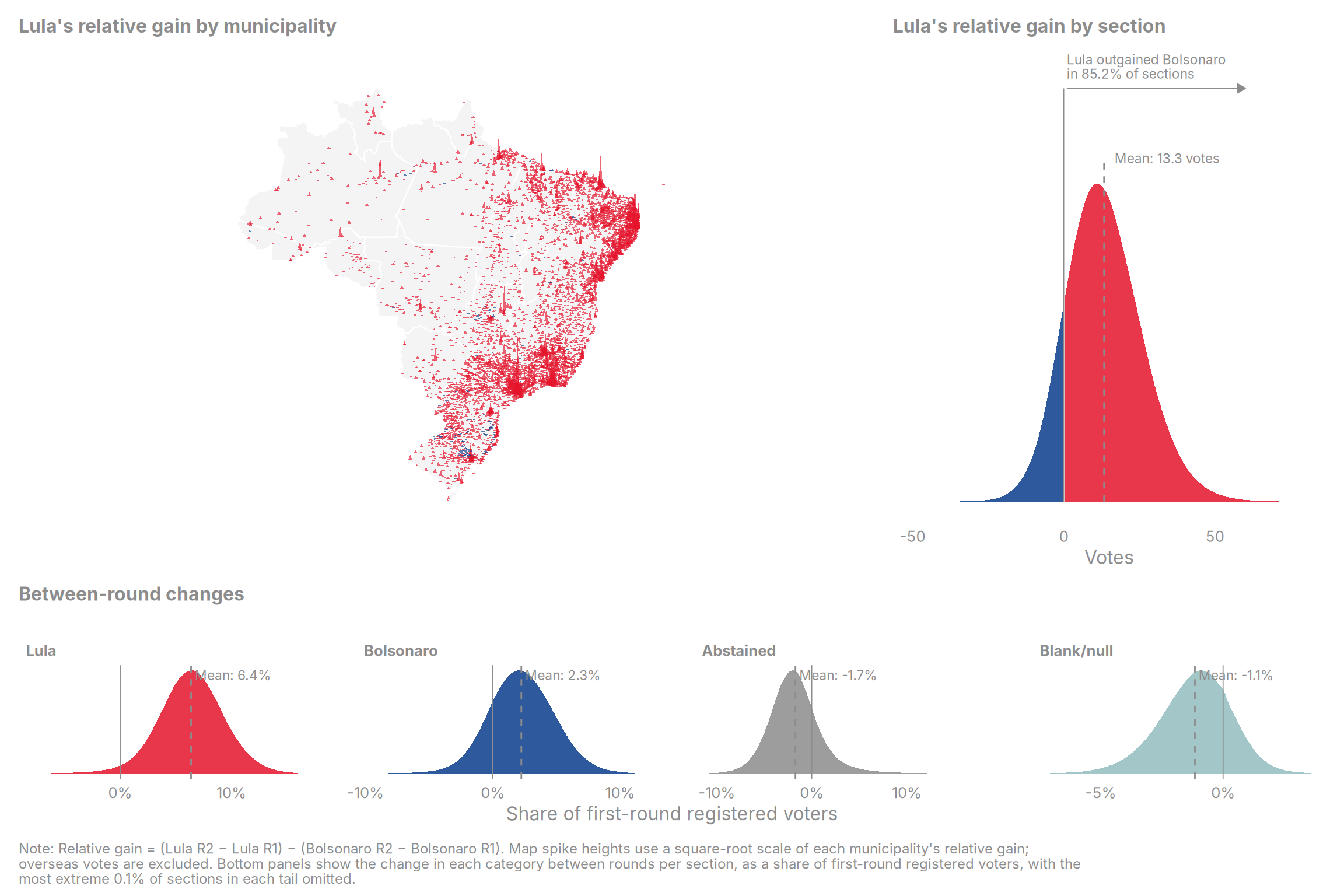
The bottom panel of Figure 6 shows that Lula gained votes almost everywhere: he lost votes in only 3% of Brazil’s nearly 500,000 sections. Abstention and spoiled-ballot voting fell on average, but not uniformly, with a sizeable proportion of sections seeing increases.
Runoff elections are, of course, designed so that third-candidate voters can reallocate their votes to the leading candidates. Therefore, we would expect both to have gained votes. The map (interactive version) and top-right density plot in Figure 6 therefore show Lula’s and Bolsonaro’s relative gains by section:
Relative gain = (LulaR2 − LulaR1) − (BolsonaroR2 − BolsonaroR1)
Lula outgained Bolsonaro in 85% of sections and, on average, gained 13 more votes per section than Bolsonaro did between rounds.4
Where did these gains come from?
The bulk of each candidate’s runoff votes likely came from their first-round voters. In theory, there are four sources from which candidates could have gained new votes between rounds:
- Mobilisation: getting people who did not vote in the first round to vote (i.e. get-out-the-vote, or GOTV).
- Spoiled-ballot persuasion: persuading voters who spoiled their ballot in the first round (by voting blank or null).
- Third-candidate persuasion: persuading voters who backed a third candidate in the first round.
- Opponent persuasion: persuading voters who backed their opponent in the first round to change their vote.
We’ve already mentioned the difficulty of attributing the result of an election to a campaign, but interpreting how votes flowed between candidates raises a second problem with the data we have.
To understand how much of Lula’s runoff vote came from each of these sources, we need to know how first-round voters voted in the second round. This type of information is exactly what the poll we used to project the second round (Table 2) contained. However, that poll represents voting intention, and we don’t (yet) have a similar poll for how voters actually changed their vote.
At this point in time, we only have election results at the aggregate level, so we can only look at changes in shares and averages. Methods for ecological inference attempt to use this information to infer how individuals changed their vote, but doing so risks making an ecological fallacy.
To be honest, I’m not an expert in these methods, but very roughly, the idea is to use areas that have very high or low rates of one type of voter in the first round to learn about what those types of voters do in the second (see the appendix for a more detailed explaination of the intuition). Crucially, to transfer information from one area to others, we have to believe that the transition rates are constant across areas (Romero et al. 2020). Unfortunately, this is a very strong assumption and everything that follows should be read with that caveat in mind.
Descriptive predictors of Lula’s gain
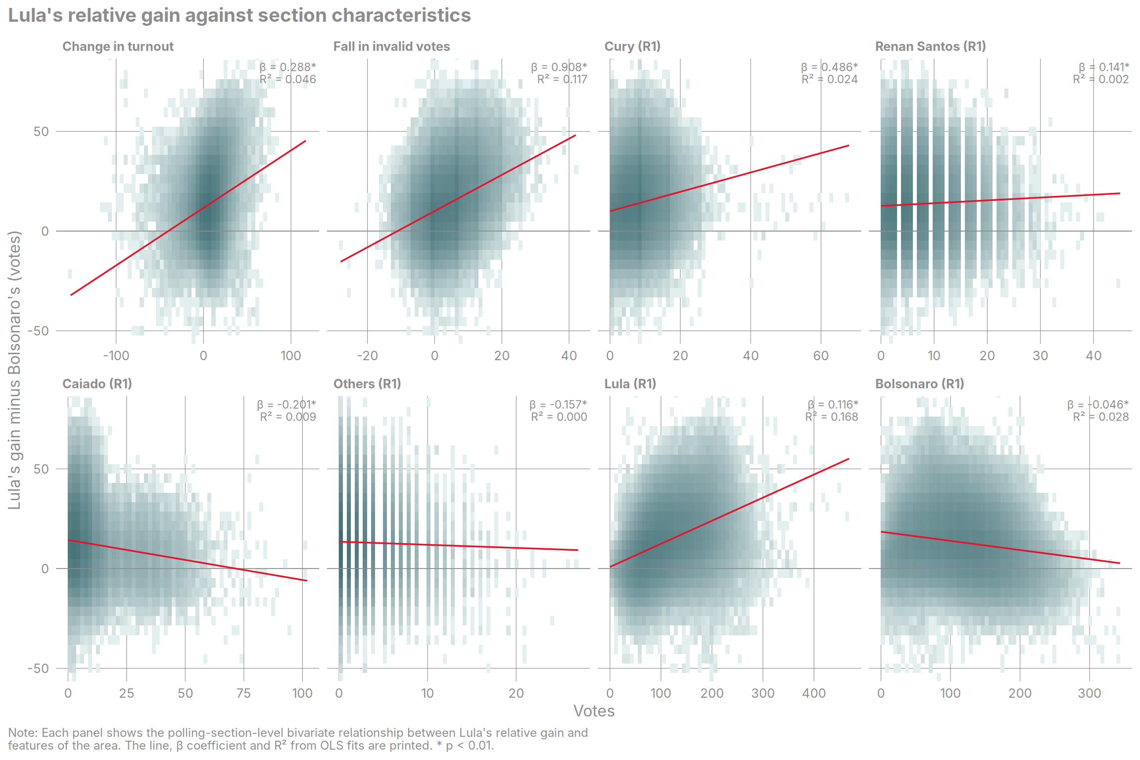
Figure 7 plots correlations between Lula’s relative gain and various predictors. It shows that Lula tended to gain more in polling sections where there were larger increases in turnout and larger decreases in blank/null votes. In sections where turnout rose by 10 more voters, Lula’s gain over Bolsonaro was about 3 votes larger; where blank/null votes fell by 10 more, about 9 votes larger.
Interestingly, Lula’s gains also appear to be stronger in sections with more first-round votes for Cury, who, recall, endorsed Bolsonaro for the runoff. For every 10 more first-round Cury voters in a section, Lula’s relative gain was 5 votes larger.
Ecological inference model
To directly estimate vote transfers, I turn to a more formal ecological inference model. To be clear, these methods allow us to produce estimates, and can improve on simple associations, but none of them solve the fundamental problem of identifying vote shifts from aggregate data.
I use an LPHOM (“Linear Programming under Homogeneity”) estimator (see Romero et al. 2020), mostly because it is relatively fast to run and has a neat R package to implement it.5 To further ease fitting the model, I aggregate the data up to much larger electoral zones (zonas eleitorais), which contain a median of 46,651 voters.
Figure 8 shows the estimated shares of how each first-round group voted in the second round (see the appendix for a comparison to the polling estimates we used earlier).
The model suggests that both candidates retained almost all of their first-round voters. Voters who spoiled their ballot are estimated to have overwhelmingly split to Lula in the second round, alongside voters for Cury, Renan Santos and the left-wing third candidates. Amongst those who abstained, we predict 8% voted for Lula and 3% for Bolsonaro. Whilst these are small percentages, remember that this group is much bigger than any third candidate’s vote.
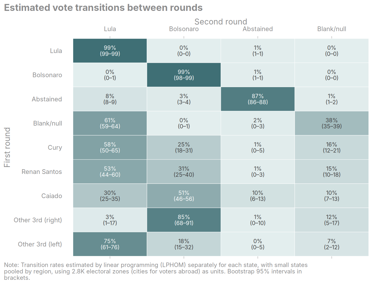
Building on that intuition, multiplying these shares by each group’s first-round size gives us an estimate of the composition of Lula’s second-round vote, shown in Figure 9.
Figure 9 suggests that, aside from retained first-round voters, Lula made most of his gains from third-candidate and spoiled-ballot persuasion. The estimated votes gained from these two groups of voters alone would have been enough to swing it for Lula. These models match the patterns suggested in Figure 7, where Lula’s gains correlated most strongly with falls in blank/null votes, Cury vote share and changes in turnout. Mobilisation is estimated to have added 2.7M votes which, whilst sizeable, would not have been enough alone to win the runoff.
Why did third-candidate and blank/null voters switch to Lula?
What might explain this pattern? A chunk of these voters may have been using the first round as an opportunity to send a clear, and potentially costly, signal to Lula that they were dissatisfied with him, but disliked Bolsonaro more, so voted tactically for Lula in the runoff.
These voters are both groups who showed up to vote, but deliberately chose against the top two in some way. This explanation makes most sense for voters who voted for a third candidate in the first round. The runoff is only called if no candidate reaches 50% of valid votes. Voting for a third candidate counts as a valid vote and increases the chance of a runoff round. Spoiling the ballot risks one of the top-two candidates winning in the first round. However, since the runoff system was introduced, all Brazilian elections but two presidential elections (1994 and 1998) have gone to a runoff, so voters probably don’t perceive this as a big risk.
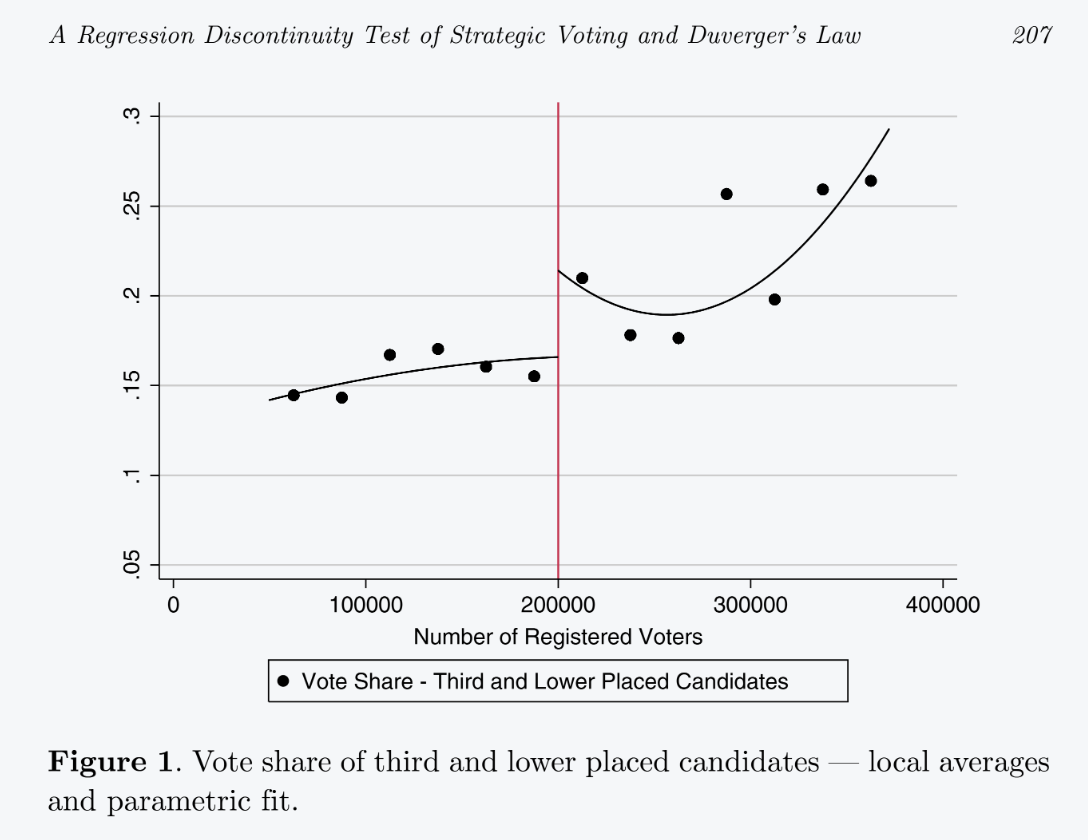
Political science research does show that Brazilian voters use the runoff system strategically. In mayoral elections, there is only a runoff in municipalities with more than 200K voters. A paper by Fujiwara (2011) uses this cut-off to compare how many votes third candidates get in municipalities just above and below this threshold. The reproduced figure from the paper (Figure 10) shows evidence that Brazilian voters do indeed use the runoff system in this way.
Concluding thoughts
Using the data we have available now, it appears that Lula’s turnaround of the 2026 Brazilian presidential election was driven primarily by third-candidate and spoiled-ballot voters voting tactically to keep Bolsonaro out.
The models I’ve used to estimate this rely on very strong assumptions about electoral behaviour. Ultimately, we can only assess their usefulness in light of additional individual-level survey data when it is released.
Even if we take these results at face value, it doesn’t mean that mobilisation didn’t matter. The increase in turnout between rounds was unprecedented and appears to have gained a substantial portion of votes.
Additionally, whilst I’ve spoken about the source of second-round votes, we don’t know what caused first-round voters to reallocate their votes to Lula. There are many potential causes, all of which likely played some role. The scale of Lula’s between-round ground and social media campaign was remarkable. Equally, between the rounds, Lula promised substantial additional spending targeting entrepreneurs and welfare recipients, and the government brought forward welfare payments. Lula was also seen to have performed well at key moments in the TV debates. These elements of what scholars of American campaigns would call the “air war” could have played an equally or more important role in securing votes.
What does this mean for Lula’s presidency? Governing will already be challenging, given the big gains for right-wing parties in legislative elections, which coincided with the first round. If we buy the tactical-voting story of the turnaround, then Lula’s presidential electoral coalition is fragile and may not survive a less extreme opponent.
Sources for third-candidate endorsements
| Candidate | Party | Second-round endorsement | Source |
|---|---|---|---|
| Augusto Cury | Avante | Flávio Bolsonaro | Correio 24 Horas |
| Ronaldo Caiado | PSD | Flávio Bolsonaro | Correio 24 Horas |
| Romeu Zema | Novo | Flávio Bolsonaro | Correio 24 Horas |
| Clariana Barão | DC | Flávio Bolsonaro | Correio 24 Horas |
| Wilson Grassi | Democrata | Flávio Bolsonaro | Gazeta do Povo |
| Renan Santos | Missão | Neutral | Correio 24 Horas |
| Samara Martins | UP | Lula | Correio 24 Horas |
| Edmilson Costa | PCB | Lula | Correio 24 Horas |
| Hertz Dias | PSTU | Lula | Correio 24 Horas |
| Rui Costa Pimenta | PCO | Null vote | Correio 24 Horas |
| Leonardo Avalanche | PRTB | None (withdrew before first round) | Mais Goiás |
Polling of third-candidate voters
In a survey by Quaest, run between 10 and 13 October (source), respondents were asked whether and how they voted on 4 October, and their second-round voting intention (Table 2).
| First-round group (share of sample) | Bolsonaro | Lula | Undecided | Blank/null/won’t vote |
|---|---|---|---|---|
| Caiado (2%) | 42% | 23% | 2% | 33% |
| Renan Santos (2%) | 40% | 14% | 3% | 43% |
| Augusto Cury (2%) | 30% | 34% | 6% | 30% |
| Others (<1%) | 38% | 33% | 7% | 22% |
| Abstained or blank/null | 38% | 43% | 2% | 17% |
The poll also reported runoff vote intention among voters who had abstained or spoiled their ballot in the first round. 43% said they would vote for Lula and 38% for Bolsonaro. However, we might have reason to doubt these estimates. Only 17% of them said they would abstain or spoil their ballot again.
It is unclear what population this group really represents, which makes using it for extrapolation difficult. It is very unlikely to be a representative sample of all first-round abstainers and spoiled-ballot voters.
If it were, it would imply a runoff valid-vote share of 93.6%, whereas the actual figure was 78.1%. Given how hard it is to reach non-voters in general, and especially in a compulsory-voting context, I assume this subgroup mostly represents voters who spoiled their ballot.
It may also include 16- and 17-year-olds, for whom voting is voluntary. For the projection, I therefore apply these figures only to first-round blank and null votes. Even applying them to abstainers as well, the projection still has Bolsonaro winning (see Figure 11).
How do the ecological inference and between-round polling estimates compare?
Figure 12 compares transition rate estimates from our ecological inference model and the between-round poll. The most striking difference is that the ecological inference estimates predict that almost no blank or null votes went to Bolsonaro. The ecological inference estimates also suggest far more Renan Santos voters split to Lula than predicted.
Neither of these is a “ground truth” of how voters voted in the second round. The poll may be based on an unrepresentative sample, or have missed changes that happened closer to the second round. The ecological inferences are subject to strong assumptions, as discussed.
We will have to see which, if either, was closer once high-quality individual-level post-election polling is released.
My understanding of the intuition behind ecological inference
We are trying to discover what proportion of each first-round group voted for each option in the second round (i.e. the empty cells in Table 3). This would let us see where Lula got his additional votes from: multiplying the size of each first-round group by the proportion of that group who voted for Lula in the second round. However, with only aggregate vote counts, we can’t observe these proportions directly.
| First round ↓ / Second round → | Lula | Bolsonaro | Blank/null | Abstained | First-round total |
|---|---|---|---|---|---|
| Lula | ? | ? | ? | ? | 53.9M |
| Bolsonaro | ? | ? | ? | ? | 56.1M |
| Third candidates | ? | ? | ? | ? | 9.3M |
| Blank/null | ? | ? | ? | ? | 6.0M |
| Abstained | ? | ? | ? | ? | 33.5M |
| Second-round total | 64.3M | 59.8M | 4.2M | 30.5M | 158.8M |
From aggregate data, we can see the totals from each round (the margins), but not the combinations of first- and second-round choices (the cells).
The idea of ecological inference is to use variation across areas to estimate these cells. Areas with a very high or very low share of a group tell us most about how that group behaves. If we assume that people transfer their votes at similar rates everywhere (a strong assumption), we can in principle recover the national transition rates. The toy example below shows an extreme version of this, and how it can go wrong.
Example
Imagine there are only two candidates, A and B, and everyone votes in both rounds. There are three areas with 1,000 voters each. We want to know what share of each first-round group voted A in the second round. The true rates, which we never get to see, are:
- 90% of first-round A voters vote A again, and 10% switch to B.
- 30% of first-round B voters switch to A, and 70% stay with B.
Across the three areas, we observe the totals for each round, but not how many voters switched between rounds (Table 4).
| Round 1 ↓ / Round 2 → | A | B | Round 1 total |
|---|---|---|---|
| A | ? | ? | 1,500 |
| B | ? | ? | 1,500 |
| Round 2 total | 1,800 | 1,200 | 3,000 |
These totals are consistent with many possible transition rates, so we can’t recover the true rates from this information alone. For example, all 1,500 first-round A voters could have voted A again, with 300 B voters switching to A. Or 1,200 A voters could have stayed, with 600 B voters switching. Both give exactly the same totals.
Now let’s break the results down into the three areas. Imagine that in the first round one area voted 100% for A, another voted 0% for A (i.e. 100% for B), and the third was split 50/50 (Table 5).
| Area | First-round A share | Second-round A votes | Second-round A share |
|---|---|---|---|
| 1 | 100% | 900 | 90% |
| 2 | 0% | 300 | 30% |
| 3 | 50% | 600 | 60% |
Area 1 contains only first-round A voters, so we can tell that 90% of them voted A again. Area 2 contains only first-round B voters, so A’s 30% share there in the second round means 30% of B voters must have switched to A.
If the rates are the same everywhere, then in Area 3, 90% of first-round A voters and 30% of first-round B voters vote A. That gives A a second-round share of 0.5 × 90% + 0.5 × 30% = 60%. All three areas lie on a straight line (Figure 13). Its value where first-round A share is 0% is the B → A rate, and its value at 100% is the A → A rate.
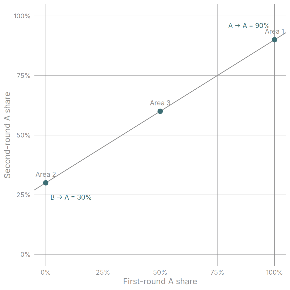
In real data we have far more areas, but we almost never see areas made up entirely of one group. Instead, we fit a line through many mixed areas and extend it to estimate the rates at each end, where the group makes up 0% or 100% of voters. This logic depends on transition rates being the same across areas.
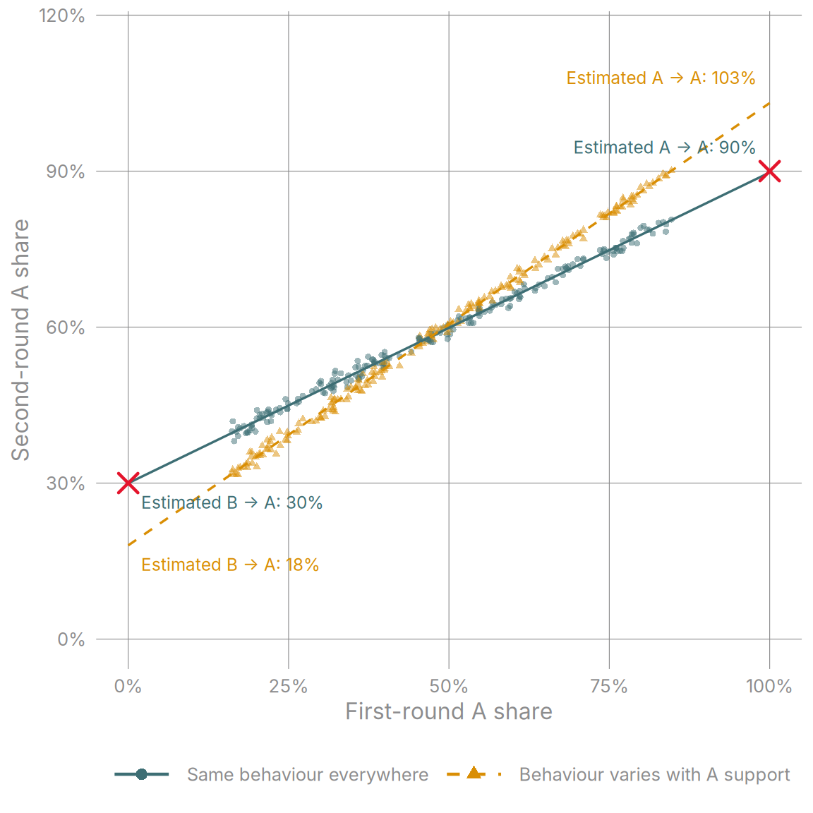
Figure 14 shows simulated data from 200 areas in two worlds. In green, the circles and solid line show what we would observe if transition rates were the same everywhere. Extending the line to 0% and 100% first-round A share correctly recovers the true rates (the red crosses). In orange, the triangles and dashed line show a world with the same average rates, but where behaviour varies with local support: where A did well, A voters were more loyal and B voters were more likely to switch to A.
Extending this line underestimates the B → A rate (18% rather than 30%) and overestimates the A → A rate (103% rather than 90%).
This example also shows how linear extrapolation can lead to implausible estimates (we estimate a transition rate for A → A of 103%).
Crucially, the orange points still sit on a tidy straight line, so nothing in the data warns us that something is wrong. The ends of the line tell us how voters behave in the most A-heavy and B-heavy areas, and in this world those voters aren’t typical.
The methods used for ecological inference in practice are far more sophisticated than this. They can control for background features of places, partly relax the assumption that transition rates are the same everywhere, and rule out impossible estimates. But fundamentally, none of them can get around the need to make some strong assumptions.
References
Broockman, David, and Joshua Kalla. 2016. “Durably Reducing Transphobia: A Field Experiment on Door-to-Door Canvassing.” Science 352 (6282): 220–24. https://doi.org/10.1126/science.aad9713.
Dyer, Geoff, Michael Pooler, and Langella Beatriz. 2026. “How Lula Turned His Election Fortunes Around in Three Weeks.” Financial Times. https://www.ft.com/content/629894c7-e753-4e77-9794-c363c64dce9a.
Foos, Florian, and Lennard Metson. 2026. “Election Campaigns.” Preprint, October. https://doi.org/https://osf.io/preprints/socarxiv/sf7cv_v1.
Fujiwara, Thomas. 2011. “A Regression Discontinuity Test of Strategic Voting and Duverger’s Law.” Quarterly Journal of Political Science 6 (3): 197–233. https://doi.org/10.1561/100.00010037.
Kalla, and Broockman. 2023. “Which Narrative Strategies Durably Reduce Prejudice? Evidence from Field and Survey Experiments Supporting the Efficacy of Perspective‐getting.” American Journal of Political Science, ajps.12657. https://doi.org/10.1111/ajps.12657.
Kreiss, Daniel. 2016. Prototype Politics: Technology-Intensive Campaigning and the Data of Democracy. New York, NY: Oxford University Press.
McKenna, Elizabeth, and Hahrie Han. 2014. Groundbreakers: How Obama’s 2.2 Million Volunteers Transformed Campaigning in America. New York, NY: Oxford University Press.
Morales, Andrés. 2026. “Punishment for Not Voting in Brazil and How to Fix It.” The Rio Times. https://www.riotimesonline.com/punishment-for-not-voting-in-brazil-2026/.
Romero, Rafael, Jose M. Pavía, Jorge Martín, and Gerardo Romero. 2020. “Assessing Uncertainty of Voter Transitions Estimated from Aggregated Data. Application to the 2017 French Presidential Election.” Journal of Applied Statistics 47 (13): 2711–36. https://doi.org/10.1080/02664763.2020.1804842.
Wikipedia. n.d.a. “2026 Brazilian General Election.” Wikipedia. Accessed October 26, 2026. https://en.wikipedia.org/wiki/2026_Brazilian_general_election#Campaign.
———. n.d.b. “André Janones.” Wikipedia. Accessed October 26, 2026. https://en.wikipedia.org/wiki/Andr%C3%A9_Janones.
Footnotes
Janones is not a member of Lula’s party, having left in 2015. But his new party, REDE, formed part of Lula’s pre-election coalition, “O Brasil está pronto para mais” (Brazil Ready for More) (Wikipedia n.d.a, n.d.b).↩︎
Voters vote by entering a candidate’s number on the voting machine. A “blank” vote is when a voter enters no number and a “null” vote is when they enter a number not associated with any candidate.↩︎
By default, the projection uses Quaest’s transfer rates, with undecided respondents redistributed proportionally. First-round abstainers are held as abstaining, and first-round Lula and Bolsonaro voters are assumed to stay loyal.↩︎
This page shows an interactive version of the map and a lookup table for vote shares and gains for each municipality and city for voters abroad.↩︎
Admittedly, this is not my finest estimator-selection moment… sorry! But similar analyses (e.g. Daniel Schteingart) by people with higher standards and bigger computers, using different estimators, appear to concur with what I find.↩︎